

What is OTTM?
OTTM stands for Ocean Tracer Transport Model. It may also be called as Offline Tracer Transport Model, but originally it was named as shown in the first form.
History of OTTM:
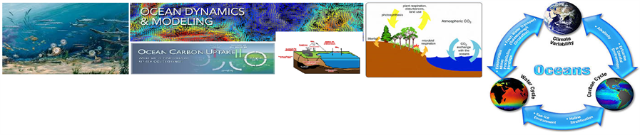
OTTM is developed to conduct researches on the ocean carbon cycle. It was initially developed in the modeling group of GOSAT-project operating at the National Institute for Environmental Studies (NIES), Tsukuba, Japan. The first version of the model was developed and tested in 2006 and published in 2008. For any questions and comments on the model and development, please contact valsala@tropmet.res.in
What does OTTM do?
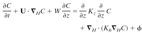
OTTM calculates the evolution of a prognostic passive tracer in the ocean by solving the advection-diffusion-mixing-source-sink equation of any scalar tracer. OTTM operates on pre-determined currents and other physical parameters of the sea, as well as the atmosphere. Therefore, OTTM is an offline model, meaning that it requires a 4-dimensional data of ocean currents, temperature, salinity, and other physical parameters to drive the model. OTTM solves only the scalar tracer equation. The following is the general form of the scalar tracer equation solved in OTTM.
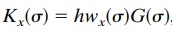
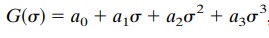
In the above equation, C represents the scalar tracer (or passive tracer). The U represents the 4-dimensional ocean velocities, the 'de' operator represents the horizontal gradient operator, Kz represents the vertical mixing coefficients, Kh represents the horizontal diffusion coefficients, Φ represents the tracer source or sink term. In addition to the above general form of the equation, OTTM specifically includes other processes of tracer evolution in the ocean, such as isopycnal diffusion and eddy-induced transports. These two terms are calculated based on the following general form.
The above term is added as bolus velocities into the first equation to account for the eddy induced transport. In a verbal format, the OTTM solves the following processes,
Tracer evolution = advection + convection + vertical mixing + horizontal diffusion + eddy induced transport + isopycnal diffusion + source + sink.
What is the difference between OTTM and conventional Ocean General Circulation Model (OGCM)?
OTTM does not solve momentum (i.e., velocities) and active tracer (i.e., temperature, salinity, and density) equations like in OGCM. Instead, OTTM borrows these essential parameters from a foreign model output or an ocean reanalysis data and utilize them to evolve a passive tracer or scalar in the ocean. Such models that operate on pre-determined circulations are generally called offline models.
What are the variables required externally, and what are diagnosed internally in OTTM?
OTTM require zonal velocity(u), meridional velocity (v), temperature (t), salinity (s) as 4-dimensional variables. Most of the foreign model outputs are available only in the above four parameters. Essential parameters such as seasonal vertical mixing coefficients are seldom available from the parent model. Therefore OTTM is designed to calculate its mixing coefficients with the additional information of surface forcing parameters. They are zonal wind stress (Tx), meridional wind stress (Ty), surface shortwave flux, net heat flux, and precipitation-evaporation fluxes. With the help of these OTTM, calculate the vertical mixing coefficient based on KPP-parameterization. Vertical velocity is calculated within OTTM by respecting the principles of the continuity equation.
How is OTTM coded?
OTTM is coded in simple Fortran-77 language with an essential parallel environment. The model runs only in parallel or cluster computers. The geometry of the model is in spherical coordinates with poles located precisely over the geometric poles the earth. It is a finite volume model in which the coordinates are in x,y,z directions. The Arakawa-B grid is used for the horizontal staggering of grids. The vertical coordinates are in z-levels.
What are the applications of OTTM?
OTTM can be used to find four-dimensional evolutions of any passive tracers (scalars) in the ocean. The tracers can be artificial dye age tracers or any other meaningful biogeochemical elements. Therefore OTTM can be readily used as a biogeochemical model.
What are the environments required to run/use OTTM?
a. Technically, a parallel computing environment or cluster of computers is required to run OTTM. It cannot be run in a single processor. It requires a multi-processor facility.
b. An input offline data of ocean velocities, temperature, salinity, and other essential parameters are required. Usually, these can be monthly data from a foreign model output or an ocean reanalysis data. OTTM interpolates the offline inputs into model time steps to find the evolution of tracers.
c. Input data are preferably from a model output, which is also run under a staggered B-grid configuration. Otherwise, OTTM calculates the B-grid data, which may conserve mass in different volume cells than in the parent input data.
d. All the input data should be converted to a model friendly format. OTTM accepts binary sequential access unformatted files created in Fortran. Outputs will be available in NetCDF format.
What are the essential tests for the OTTM?
OTTM can be tested for its spherical geometry based on a simple test of sphere rotation. OTTM is primarily coded in spherical coordinates with a constant radius of the earth. Therefore, a test velocity is generated, as if a sphere is rotating concerning an axle passing through its center. For such rotations, each point on the surface of the area will have a specific velocity vector, which can be written down in simple spherical coordinate trigonometric equations of sin and cos functions. After resolving u, v (i.e., zonal and meridional velocities), they are used to run the OTTM for a test case. In this sphere rotation case, the horizontal speeds are non-convergent. In this 2-dimensional sphere rotation experiment, any tracer initialized in OTTM should rotate as if it is a sticker on a rotating solid sphere. This property is a powerful tool to evaluate the geometry of the model and its fidelity and estimate the numerical errors and other statistics.
How do we validate the results of OTTM in a real application case?
OTTM or any transport model needs a thorough validation of results. OTTM is usually validated by simulating the Chlorofluorocarbon (CFC) in the ocean. The CFC has been emitted to the atmosphere since the 1930s. The atmospheric record of CFC is available from the 1930s. Initially, the sea had zero CFC concentrations. Since the 1930s, the CFC concentration in the ocean is increasing, until recently, due to the industrial emissions of CFC.
CFC simulations can verify OTTM results. For this purpose, the OTTM is used to simulate the oceanic CFC from 1930 and continue the simulation until 1995 or 2000. A global survey of CFC during the 1990s is available as observational data. The simulated CFC concentration of the model year 1995 can be compared with the global mean observations. For an accurate transport model, the model CFC should match with the observations. The model error can be estimated in this way.
What are the works so far done using OTTM?
OTTM has been used, so far, for the following purposes.
a. CFC-11 simulation, validation and interannual variability of CFC-11 sinks
In Valsala et al. (2008), we validated the OTTM using CFC-11 simulations. Oceanic concentrations of CFC-11 were simulated from 1938 to 2000 using offline input data from GFDL reanalyses. This work reported the design and validation of OTTM by simulation of CFC-11.
In the following study, Valsala and Maksyutov, (2010a) have used OTTM to investigate the interannual variability of CFC-11 sink in the ocean. The significant finding was that the CFC sink variability of the ocean is tied to climate variabilities such as El Nino and other significant climate anomalies. The ocean's capacity to sequestrate CFC is reducing due to its saturation in the upper parts of the sea. Slow transport of CFC from ocean thermocline to subsurface causes congestion of CFC11 in the thermocline and slowdown of continued uptake of CFC-11 by the ocean.
b. Carbon cycle simulation and air-sea CO2 flux assimilation.
In Valsala and Maksytov (2010b), the OTTM was used to simulate the carbon cycle in the ocean-based up on a simple biogeochemical model. The target was to find out the contemporary CO2 fluxes between the atmosphere and the sea. We used the OCMIP-II type simple abiotic model for the carbon chemistry and a phosphate-dependent one-component ecosystem model for the biology. In addition to the simulation of CO2 fluxes, we assimilated the surface ocean pCO2 of the model with the ship-based observations. We synthesized a nine-year of air-sea CO2 flux data from 1996 to 2004 in this study. The OTTM is used for assimilation in a 4D-variational approach. The 'adjoint' of the forward model was simply estimated with reversed currents of the offline input data, and the integrations were carried out from the endpoint to the starting point. The assimilated air-sea CO2 flux data from 1996 to 2004 is available at http://cdiac.ornl.gov/oceans/CO2_Flux_1996_2004.html and a long record of 1980 to 2010 at http://apdrc.soest.hawaii.edu/datadoc/co2_flux.php
c. Pathways of water masses in the ocean and its variability.
OTTM can be used to simulate ideal dye tracer in response to a source kept at any point in the ocean. This property is used to trace the Indonesian Throughflow (ITF) in the Indian Ocean from 1950 to 2000. The target was to find out the interannual variability of pathways of the ITF in the Indian Ocean. In this case, two sets of simulations were done using OTTM. In the control case, an ideal tracer from the ITF origin region is traced for 50 years using monthly circulations of offline input data. In a second run, the OTTM is simulated for the same source of tracer but with climatological monthly mean repeatedly flows for 50 years. The difference between the control-run and the climatological-run gives the oscillating patterns of tracers in the ocean. They come from the interannual variability in the circulation. An EOF method is employed to find a significant dancing pattern of the dye tracers. They are interpreted as the interannual variability in the pathways of the ITF. The results were published in Valsala et al. (2010c).
In a complementary study, OTTM was used in adjoint mode to detect the origin and pathway variability of ITF in the Pacific Ocean. The adjoint model means the backward simulation of tracers with a reversed currents (input current data is multiplied by negative 1 to change the direction of flow) and integrate the model from an endpoint (year-2000) to starting point (year-1950). It gives the origin of ITF in the Pacific Ocean. The above sets of experiments were done in the adjoint OTTM model, and pathway variability of the source of ITF in the Pacific Ocean was found. Results were published in Valsala et al. (2011).
What are the potential (future) usages of OTTM?
1. Dispersion of dye in the ocean. It can be used to find pollution transport in the sea, such as oil-spillage.
2. Dispersion of biological elements such as Larvae, microbial, and fish-eggs.
3. Identifying a suitable location in the ocean for waste material dumping from where they never or least surfaces after disposal. This can be used in artificial carbon sequestration projects.
4. Biogeochemistry and Carbon cycle simulations of global oceans.
5. Adjoints and variational data assimilation.
OTTM stands for Ocean Tracer Transport Model. It may also be called as Offline Tracer Transport Model, but originally it was named as shown in the first form.
History of OTTM:
OTTM is developed to conduct researches on the ocean carbon cycle. It was initially developed in the modeling group of GOSAT-project operating at the National Institute for Environmental Studies (NIES), Tsukuba, Japan. The first version of the model was developed and tested in 2006 and published in 2008. For any questions and comments on the model and development, please contact valsala@tropmet.res.in
What does OTTM do?
OTTM calculates the evolution of a prognostic passive tracer in the ocean by solving the advection-diffusion-mixing-source-sink equation of any scalar tracer. OTTM operates on pre-determined currents and other physical parameters of the sea, as well as the atmosphere. Therefore, OTTM is an offline model, meaning that it requires a 4-dimensional data of ocean currents, temperature, salinity, and other physical parameters to drive the model. OTTM solves only the scalar tracer equation. The following is the general form of the scalar tracer equation solved in OTTM.
In the above equation, C represents the scalar tracer (or passive tracer). The U represents the 4-dimensional ocean velocities, the 'de' operator represents the horizontal gradient operator, Kz represents the vertical mixing coefficients, Kh represents the horizontal diffusion coefficients, Φ represents the tracer source or sink term. In addition to the above general form of the equation, OTTM specifically includes other processes of tracer evolution in the ocean, such as isopycnal diffusion and eddy-induced transports. These two terms are calculated based on the following general form.
The above term is added as bolus velocities into the first equation to account for the eddy induced transport. In a verbal format, the OTTM solves the following processes,
Tracer evolution = advection + convection + vertical mixing + horizontal diffusion + eddy induced transport + isopycnal diffusion + source + sink.
What is the difference between OTTM and conventional Ocean General Circulation Model (OGCM)?
OTTM does not solve momentum (i.e., velocities) and active tracer (i.e., temperature, salinity, and density) equations like in OGCM. Instead, OTTM borrows these essential parameters from a foreign model output or an ocean reanalysis data and utilize them to evolve a passive tracer or scalar in the ocean. Such models that operate on pre-determined circulations are generally called offline models.
What are the variables required externally, and what are diagnosed internally in OTTM?
OTTM require zonal velocity(u), meridional velocity (v), temperature (t), salinity (s) as 4-dimensional variables. Most of the foreign model outputs are available only in the above four parameters. Essential parameters such as seasonal vertical mixing coefficients are seldom available from the parent model. Therefore OTTM is designed to calculate its mixing coefficients with the additional information of surface forcing parameters. They are zonal wind stress (Tx), meridional wind stress (Ty), surface shortwave flux, net heat flux, and precipitation-evaporation fluxes. With the help of these OTTM, calculate the vertical mixing coefficient based on KPP-parameterization. Vertical velocity is calculated within OTTM by respecting the principles of the continuity equation.
How is OTTM coded?
OTTM is coded in simple Fortran-77 language with an essential parallel environment. The model runs only in parallel or cluster computers. The geometry of the model is in spherical coordinates with poles located precisely over the geometric poles the earth. It is a finite volume model in which the coordinates are in x,y,z directions. The Arakawa-B grid is used for the horizontal staggering of grids. The vertical coordinates are in z-levels.
What are the applications of OTTM?
OTTM can be used to find four-dimensional evolutions of any passive tracers (scalars) in the ocean. The tracers can be artificial dye age tracers or any other meaningful biogeochemical elements. Therefore OTTM can be readily used as a biogeochemical model.
What are the environments required to run/use OTTM?
a. Technically, a parallel computing environment or cluster of computers is required to run OTTM. It cannot be run in a single processor. It requires a multi-processor facility.
b. An input offline data of ocean velocities, temperature, salinity, and other essential parameters are required. Usually, these can be monthly data from a foreign model output or an ocean reanalysis data. OTTM interpolates the offline inputs into model time steps to find the evolution of tracers.
c. Input data are preferably from a model output, which is also run under a staggered B-grid configuration. Otherwise, OTTM calculates the B-grid data, which may conserve mass in different volume cells than in the parent input data.
d. All the input data should be converted to a model friendly format. OTTM accepts binary sequential access unformatted files created in Fortran. Outputs will be available in NetCDF format.
What are the essential tests for the OTTM?
OTTM can be tested for its spherical geometry based on a simple test of sphere rotation. OTTM is primarily coded in spherical coordinates with a constant radius of the earth. Therefore, a test velocity is generated, as if a sphere is rotating concerning an axle passing through its center. For such rotations, each point on the surface of the area will have a specific velocity vector, which can be written down in simple spherical coordinate trigonometric equations of sin and cos functions. After resolving u, v (i.e., zonal and meridional velocities), they are used to run the OTTM for a test case. In this sphere rotation case, the horizontal speeds are non-convergent. In this 2-dimensional sphere rotation experiment, any tracer initialized in OTTM should rotate as if it is a sticker on a rotating solid sphere. This property is a powerful tool to evaluate the geometry of the model and its fidelity and estimate the numerical errors and other statistics.
How do we validate the results of OTTM in a real application case?
OTTM or any transport model needs a thorough validation of results. OTTM is usually validated by simulating the Chlorofluorocarbon (CFC) in the ocean. The CFC has been emitted to the atmosphere since the 1930s. The atmospheric record of CFC is available from the 1930s. Initially, the sea had zero CFC concentrations. Since the 1930s, the CFC concentration in the ocean is increasing, until recently, due to the industrial emissions of CFC.
CFC simulations can verify OTTM results. For this purpose, the OTTM is used to simulate the oceanic CFC from 1930 and continue the simulation until 1995 or 2000. A global survey of CFC during the 1990s is available as observational data. The simulated CFC concentration of the model year 1995 can be compared with the global mean observations. For an accurate transport model, the model CFC should match with the observations. The model error can be estimated in this way.
What are the works so far done using OTTM?
OTTM has been used, so far, for the following purposes.
a. CFC-11 simulation, validation and interannual variability of CFC-11 sinks
In Valsala et al. (2008), we validated the OTTM using CFC-11 simulations. Oceanic concentrations of CFC-11 were simulated from 1938 to 2000 using offline input data from GFDL reanalyses. This work reported the design and validation of OTTM by simulation of CFC-11.
In the following study, Valsala and Maksyutov, (2010a) have used OTTM to investigate the interannual variability of CFC-11 sink in the ocean. The significant finding was that the CFC sink variability of the ocean is tied to climate variabilities such as El Nino and other significant climate anomalies. The ocean's capacity to sequestrate CFC is reducing due to its saturation in the upper parts of the sea. Slow transport of CFC from ocean thermocline to subsurface causes congestion of CFC11 in the thermocline and slowdown of continued uptake of CFC-11 by the ocean.
b. Carbon cycle simulation and air-sea CO2 flux assimilation.
In Valsala and Maksytov (2010b), the OTTM was used to simulate the carbon cycle in the ocean-based up on a simple biogeochemical model. The target was to find out the contemporary CO2 fluxes between the atmosphere and the sea. We used the OCMIP-II type simple abiotic model for the carbon chemistry and a phosphate-dependent one-component ecosystem model for the biology. In addition to the simulation of CO2 fluxes, we assimilated the surface ocean pCO2 of the model with the ship-based observations. We synthesized a nine-year of air-sea CO2 flux data from 1996 to 2004 in this study. The OTTM is used for assimilation in a 4D-variational approach. The 'adjoint' of the forward model was simply estimated with reversed currents of the offline input data, and the integrations were carried out from the endpoint to the starting point. The assimilated air-sea CO2 flux data from 1996 to 2004 is available at http://cdiac.ornl.gov/oceans/CO2_Flux_1996_2004.html and a long record of 1980 to 2010 at http://apdrc.soest.hawaii.edu/datadoc/co2_flux.php
c. Pathways of water masses in the ocean and its variability.
OTTM can be used to simulate ideal dye tracer in response to a source kept at any point in the ocean. This property is used to trace the Indonesian Throughflow (ITF) in the Indian Ocean from 1950 to 2000. The target was to find out the interannual variability of pathways of the ITF in the Indian Ocean. In this case, two sets of simulations were done using OTTM. In the control case, an ideal tracer from the ITF origin region is traced for 50 years using monthly circulations of offline input data. In a second run, the OTTM is simulated for the same source of tracer but with climatological monthly mean repeatedly flows for 50 years. The difference between the control-run and the climatological-run gives the oscillating patterns of tracers in the ocean. They come from the interannual variability in the circulation. An EOF method is employed to find a significant dancing pattern of the dye tracers. They are interpreted as the interannual variability in the pathways of the ITF. The results were published in Valsala et al. (2010c).
In a complementary study, OTTM was used in adjoint mode to detect the origin and pathway variability of ITF in the Pacific Ocean. The adjoint model means the backward simulation of tracers with a reversed currents (input current data is multiplied by negative 1 to change the direction of flow) and integrate the model from an endpoint (year-2000) to starting point (year-1950). It gives the origin of ITF in the Pacific Ocean. The above sets of experiments were done in the adjoint OTTM model, and pathway variability of the source of ITF in the Pacific Ocean was found. Results were published in Valsala et al. (2011).
What are the potential (future) usages of OTTM?
1. Dispersion of dye in the ocean. It can be used to find pollution transport in the sea, such as oil-spillage.
2. Dispersion of biological elements such as Larvae, microbial, and fish-eggs.
3. Identifying a suitable location in the ocean for waste material dumping from where they never or least surfaces after disposal. This can be used in artificial carbon sequestration projects.
4. Biogeochemistry and Carbon cycle simulations of global oceans.
5. Adjoints and variational data assimilation.
Group Head


Dr. Homi Bhabha Road, Pashan, Pune, 411 008, India (020) 2590 4514